Get Started
[1]:
# For installation of the necessary packages in Google Colab
try:
    import predicode as pc
except:
    # Tensorflow 2.0 must be installed manually in Google Colab
    !pip install tensorflow==2.0.0rc
    !pip install git+https://github.com/sflippl/predicode
    import predicode as pc
# lazytools just contains a few convenience functions, specifically matrix heatmaps,
# but is otherwise not necessary.
try:
    import lazytools_sflippl as lazytools
except:
    !pip install git+https://github.com/sflippl/lazytools
    import lazytools_sflippl as lazytools
In this tutorial, you will get to know the basic functionality of predicode, starting with a minimal linear predictive coding model before discussing multiple tiers, customized optimization regimens, training in batches, and the tensorboard functionality.
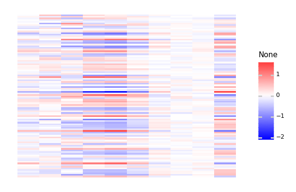
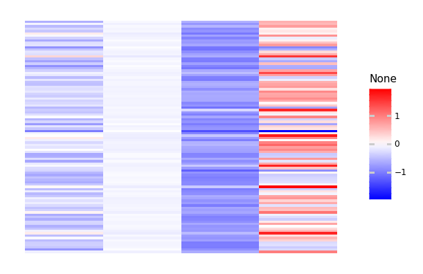
Throughout the tutorial, we will be concerned with a small artificial dataset that is normally distributed, with its principal components having exponentially decreasing variance.
[2]:
dataset = pc.datasets.decaying_multi_normal(
    dimensions=10, size=100
)
[3]:
lazytools.matrix_heatmap(dataset, pole=0)
[3]:
<ggplot: (8748327106389)>
The minimal model
As a first step, we add tiers of specified shape, in this case a ten-dimensional input layer and a four-dimensional latent layer.
[4]:
hpc_minimal = pc.Hierarchical()
hpc_minimal.add_tier(shape=(10, ))
hpc_minimal.add_tier(shape=(4, ))
Active connection: tier_1 -> tier_0
[4]:
<predicode.hierarchical.hierarchical.Hierarchical at 0x7f4e05728410>
We can inspect the current result using the summary:
[5]:
hpc_minimal.summary()
# Tier 1: tier_1

# Connection: tier_1 -> tier_0
(No tier connection defined.)

# Tier 0: tier_0
The ‘connection’ property refers to the currently activated connection, in this case the connection between tier 1 and tier 0.
This connection specifies how tier 1 is inferred from tier 0 with the observed data. The class pc.TopDownPrediction() provides a classical hierarchical predictive connection where tier 1 is used to predict tier 0 and the values of tier 1 are inferred to optimize this prediction. The provided model must be a Keras model that specifies how tier 0 is predicted from tier 1. Specifically, pc.TopDownSequential instantiates a
Sequential model.
For example, a simple linear connection is given by a sequential model consisting of single dense linear connection.
[6]:
import tensorflow.keras as keras
hpc_minimal.connection = pc.connections.TopDownSequential()
hpc_minimal.connection.add(
    keras.layers.Dense(10, input_shape=(4, ))
)
The model is now ready to be compiled:
[7]:
hpc_minimal.summary()
# Tier 1: tier_1

# Connection: tier_1 -> tier_0
Top-down prediction.
## Predictive model
Model: "sequential"
_________________________________________________________________
Layer (type)                 Output Shape              Param #
=================================================================
dense (Dense)                (None, 10)                50
=================================================================
Total params: 50
Trainable params: 50
Non-trainable params: 0
_________________________________________________________________
## Prediction error
<tensorflow.python.eager.def_function.Function object at 0x7f4e143c86d0>
## Loss function
<function mean_squared_error at 0x7f4e1de4d560>

# Tier 0: tier_0
By default, the prediction error is given by the difference between the prediction from tier 1 and the true values of tier 0, and the loss function is given by the mean squared error between the two. By compiling the model, we now specify how the states and the predictor weights are estimated.
[8]:
hpc_minimal.compile(optimizer='adam')
We can now use dataset to train the model:
[9]:
hpc_minimal.train(dataset, epochs=100)
[9]:
<predicode.hierarchical.hierarchical.Hierarchical at 0x7f4e05728410>
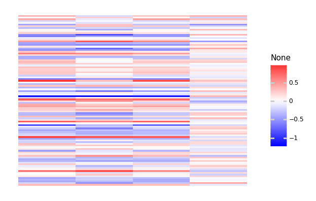
We can now inspect the estimated tiers, predictions, and prediction errors:
[10]:
lazytools.matrix_heatmap(hpc_minimal.tier(1).numpy(),
                         pole=0)
[10]:
<ggplot: (8748307531765)>
[11]:
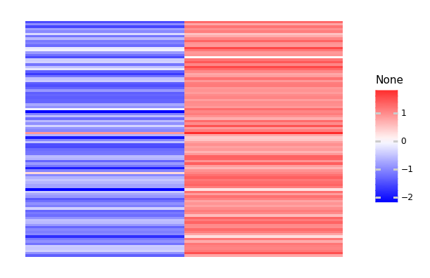
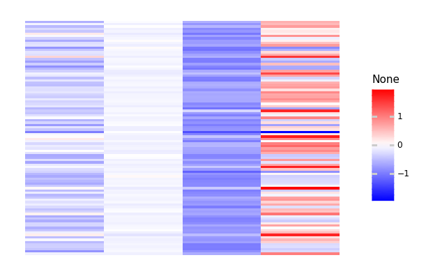
lazytools.matrix_heatmap(hpc_minimal.prediction(0).numpy(),
                         pole=0)

[11]:
<ggplot: (8748307336885)>
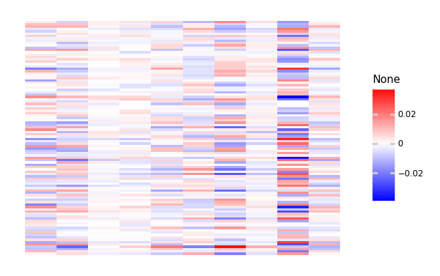
[12]:
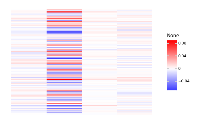
lazytools.matrix_heatmap(hpc_minimal.prediction_error(0).numpy(),
                         pole=0)
[12]:
<ggplot: (8748317225069)>
We can also inspect the estimated weights:
[13]:
hpc_minimal.connection.model.get_weights()
[13]:
[array([[ 0.4781576 ,  0.688794  ,  0.12980229,  0.5537218 ,  0.38032824,
         -0.11391962, -0.02828846,  1.0756079 ,  0.5172539 , -0.5371767 ],
        [ 1.2092746 , -0.1235444 ,  0.53653646,  0.9537554 ,  0.83324504,
         -0.46419057,  0.01348522, -1.3601234 ,  0.66269   ,  0.17493841],
        [-0.95141053,  0.06300981, -0.27511808,  0.1718974 ,  0.5279959 ,
          1.1658176 , -0.29007822, -0.20417835, -1.0425217 , -0.7889378 ],
        [ 0.7737668 ,  0.54437613, -1.2937229 ,  0.65247506,  0.03088524,
         -1.3553474 ,  0.4264841 , -1.7554736 ,  0.6602506 ,  0.57957274]],
       dtype=float32),
 array([-0.00057098, -0.00237244,  0.0034195 , -0.00104265,  0.00052802,
         0.00262731, -0.00226873, -0.00321213,  0.00054307,  0.00072796],
       dtype=float32)]
Optimization regimens
Hierarchical predictive coding must infer the latent variables and the predictor’s weights. When both are taken together, the system is oversaturated. These variables must therefore be estimated in separate stages. Usually, this is solved by the Expectation-Maximization-Algorithm, iteratively estimating states and predictor variables until convergence. This means that the usual routine of simply specifying epochs is not sufficient. Instead, convergence criteria must be specified when estimation mode should be switched.
This specification works with OptimizationRegimens. The parameter eps specifies the change at which the algorithm is assumed to have converged, and the parameter max_steps specifies and upper bound on the number of iterations.
[14]:
state_regimen = pc.regimens.OptimizerRegimen(
    optimizer=keras.optimizers.Adam(learning_rate=0.1),
    eps=1e-1,
    max_steps=100
)
[15]:
predictor_regimen = pc.regimens.OptimizerRegimen(
    optimizer=keras.optimizers.Adam(learning_rate=0.01),
    eps=1e-3,
    max_steps=100
)
Finally, you can combine the state and predictor regimen using the class EMRegimen.
[16]:
em_regimen = pc.regimens.EMRegimen(
    state_regimen=state_regimen,
    predictor_regimen=predictor_regimen
)
As a shortcut, you can use identifiers for compilation (see help(pc.regimens.get)).
Multiple tiers
Specifying multiple tiers works in exactly the same way:
[17]:
hpc_three = pc.Hierarchical()
hpc_three.add_tier(shape=(10, ))
hpc_three.add_tier(shape=(4, ))
hpc_three.add_tier(shape=(2, ))
Active connection: tier_1 -> tier_0
Active connection: tier_2 -> tier_1
[17]:
<predicode.hierarchical.hierarchical.Hierarchical at 0x7f4dfc3892d0>
At the moment the active connection is given by the one between tier_2 and tier_1. We specify a sequential model with an intermediate nonlinearity.
[18]:
import tensorflow.keras as keras
hpc_three.connection = pc.connections.TopDownSequential(
    layers=[
        keras.layers.Dense(8, input_shape=(2, )),
        keras.layers.Activation('relu'),
        keras.layers.Dense(4)
    ]
)
We now activate the connection between tier_1 and tier_0 to specify a linear model there.
[19]:
hpc_three.activate_connection('tier_1')
Active connection: tier_1 -> tier_0
[19]:
<predicode.hierarchical.hierarchical.Hierarchical at 0x7f4dfc3892d0>
[20]:
hpc_three.connection = pc.connections.TopDownSequential(
    layers=[keras.layers.Dense(10, input_shape=(4, ),
                               use_bias=False)]
)
[21]:
hpc_three.summary()
# Tier 2: tier_2

# Connection: tier_2 -> tier_1
Top-down prediction.
## Predictive model
Model: "sequential_1"
_________________________________________________________________
Layer (type)                 Output Shape              Param #
=================================================================
dense_1 (Dense)              (None, 8)                 24
_________________________________________________________________
activation (Activation)      (None, 8)                 0
_________________________________________________________________
dense_2 (Dense)              (None, 4)                 36
=================================================================
Total params: 60
Trainable params: 60
Non-trainable params: 0
_________________________________________________________________
## Prediction error
<tensorflow.python.eager.def_function.Function object at 0x7f4e143c86d0>
## Loss function
<function mean_squared_error at 0x7f4e1de4d560>

# Tier 1: tier_1

# Connection: tier_1 -> tier_0
Top-down prediction.
## Predictive model
Model: "sequential_2"
_________________________________________________________________
Layer (type)                 Output Shape              Param #
=================================================================
dense_3 (Dense)              (None, 10)                40
=================================================================
Total params: 40
Trainable params: 40
Non-trainable params: 0
_________________________________________________________________
## Prediction error
<tensorflow.python.eager.def_function.Function object at 0x7f4e143c86d0>
## Loss function
<function mean_squared_error at 0x7f4e1de4d560>

# Tier 0: tier_0
[22]:
hpc_three.compile(optimizer=em_regimen)
[23]:
hpc_three.train(dataset, epochs=250)
[23]:
<predicode.hierarchical.hierarchical.Hierarchical at 0x7f4dfc3892d0>
We can now again examine this model:
[24]:
lazytools.matrix_heatmap(hpc_three.tier(2).numpy(), pole=0)
[24]:
<ggplot: (8748299009465)>
[25]:
lazytools.matrix_heatmap(hpc_three.prediction(1).numpy(), pole=0)
[25]:
<ggplot: (8748286785853)>
[26]:
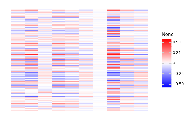
lazytools.matrix_heatmap(hpc_three.prediction_error(1).numpy(),
                         pole=0)
[26]:
<ggplot: (8748286364185)>
[27]:
lazytools.matrix_heatmap(hpc_three.tier(1).numpy(), pole=0)
[27]:
<ggplot: (8748200262345)>
Batch training
For big datasets, you can also train in batches. This means, however that you will not have retained all tiers, but only the last batch that was used.
[28]:
big_dataset = pc.datasets.decaying_multi_normal(
    dimensions=10, size=50000
)
As an example we just estimate the states for the given weights. This can be specified by only specifying a state estimator in the provided dictionary.
[29]:
hpc_minimal.compile({'states': 'adam'})
[30]:
hpc_minimal.train(big_dataset, batch_size=1000, epochs=100)
[30]:
<predicode.hierarchical.hierarchical.Hierarchical at 0x7f4e05728410>
[31]:
lazytools.matrix_heatmap(hpc_minimal.prediction(0).numpy(), pole=0)
[31]:
<ggplot: (8748299408945)>
Metrics and Tensorboard
During compilation, we can also specify metrics to keep track of:
[32]:
new_dataset = pc.datasets.decaying_multi_normal(dimensions=10, size=100)
[50]:
hpc_metrics = pc.Hierarchical(
    tiers=[(10, ), (4, )]
)
hpc_metrics.connection = pc.connections.TopDownSequential([
    keras.layers.Dense(2, input_shape=(4, )),
    keras.layers.Activation('relu'),
    keras.layers.Dense(10)
])
hpc_metrics.compile(
    pc.regimens.OptimizerRegimen(
        keras.optimizers.Adam(), max_steps=100
    ),
    metrics=[keras.metrics.MeanSquaredError(),
             keras.metrics.MeanAbsoluteError()]
)
Active connection: tier_1 -> tier_0
If you specify a log directory during training we can use Tensorboard using the summary file writer.
[51]:
import datetime
logdir = 'log/{}'.format(datetime.datetime.now())
[52]:
import tensorflow as tf
summary_writer = tf.summary.create_file_writer(logdir)
[53]:
with summary_writer.as_default():
    hpc_metrics.train(new_dataset, epochs=10)
We can now use the magic method tensorboard to inspect the progress during estimation.
%load_ext tensorboard%tensorboard --logdir log