Chapter 2 Methodology

This chapter introduces the methods with which the outlier detection algorithms are discussed in the following. It first discusses the connection between data compression, data correction, outlier labels and outlier scores, embeds methods using regression in alternatives using probabilistic modeling or clustering and then presents Z-Scoring as a simple heuristic to normalize outlier scores. Finally, evaluation of outlier scores, both in this report and in general are discussed and toy outlier datasets are introduced.

2.1 A nested account of outlier detection

Outlier detection is closely related to the fields of data compression and data correction. In fact, there is a canonical connection which will be discussed in this section. Firstly, let us produce a definition of the different general algorithms.

Definition 2.1 Consider some data $D\in\mathcal{D}^n,n\in\mathbb{N}$. An algorithm $A$ achieves

data compression if and only if it yields an encoding procedure \[E^D:\mathcal{D}\to\mathcal{C}\] (where $\mathcal{C}$ is some compressed space) and a decoding procedure \[F^D:\mathcal{C}\to\mathcal{D}.\] Consider, for instance, a large file $D\in\mathcal{D}$ where $\mathcal{D}$ is the space of files of a certain maximum size. The zipping algorithm DEFLATE uses – broadly speaking – repeating patterns in the files to reduce size by relating repeated patterns to the original pattern. For instance, the highlighted string sequence “pattern” in the last sentence occurred thrice – the latter two times, it could have been replaced by a reference to the original sequence. DEFLATE would thus produce a compressed (zipped) file $Z=E^D(D)$ which can then be decoded to yield the original data file $D = F^D(Z)$. (see Deutsch 1996)
This is an example of lossless data compression. In many cases, however, data is compressed in such a way that it cannot be entirely recovered. This is called lossy data compression. I will illustrate the procedure by a simple example. Suppose that the data consists of a set of geometrical figures. We detect that they are all rectangles and we can therefore save them by the width and height. This data compression is lossless. If we wish to compress the data even further, we might note that most rectangles are approximately squares and we can encode them by the mean of their width and height. If, for instance a rectangle of width 5.0 cm and height 6.0 cm is encoded, we save the number 5.5 (encoded). In the decoding step, we convert the number 5.5 into a square of width and height 5.5 cm. Whereas this is not exactly the rectangle we put in, we may decide that it is close enough.
data correction if and only if it yields a correction procedure \[C^D:\mathcal{D}^n\to\mathcal{D}^n\] such that $C^D(D)$ is a corrected version of $D$. In our working example, data correction would imply a different perspective on our rectangle-square-problem. Perhaps, we know that all geometrical forms are supposed to be squares but there has been some measurement error. The product could then be viewed as a computation of the most likely square that has been measured in the first place. Generally, we do not need a framework with encoding and decoding – another solution would be, for example, to assume the lesser value of width and height as the actual value of both width and height.
outlier scoring if and only if it can label each data point $d\in\mathcal{D}$ with a score that captures the dissimilarity of $d$ compared to the dataset $D$. This would, again, imply a different perspective: perhaps, not all measured forms have been squares but they have usually been approximate squares. Then, the rectangles with large differences between width and height are unusual observations and some measure like the absolute difference between width and height captures the degree to which they are outliers – their outlier score. Of course, we could also try to measure how different the corrected form (the square) is from the original form (the rectangle). The larger the difference, the larger the outlier score.
outlier labels if and only if it can label each data point $d\in\mathcal{D}$ with a binary label that indicates whether it is an outlier score or not. For instance, we might define, that those rectangles are outliers where width and height have a difference of more than 1 cm.

Outlier scoring and labeling are a part of outlier detection and we will discuss their relation in the next section. At this point, I will work out the implied relations between the different algorithms, namely:

A data compression algorithm can be used for data correction by viewing the encoded and then decoded data as corrected data.
A data correction algorithm can be used for outlier scoring by measuring the dissimilarity between the original and the corrected data.
An outlier scoring algorithm can be used for outlier labels by defining a threshold such that any data point with a larger outlier score is defined as an outlier.

This implies a nested account of outlier detection and allows us to further our understanding of capable outlier detection algorithms by regarding them as compressing and correcting algorithms. More explicitly, an unusual observation is one that cannot be compressed as much without a large margin of error, resp. one that differs a lot from its corrected version. Both perspectives therefore contribute to our understanding of outlier detection algorithms and I will regard them where appropriate.

It remains to remark that, of course, data compression algorithms are not, per se, superior to pure outlier detection algorithms just because they also induce a method of the latter category. If the latter algorithm has a better performance in detecting outliers in a certain situation, it is evidently better at this task, even if it is not capable of data compression.

2.2 Context: Probabilistic and cluster analysis for outlier detection

While this report introduces regression methods for outlier detection, this is not the only option. In its most basic form, outlier detection consists of a collection of real numbers $x_1,\dotsc, x_n$ and the suspicious data points are “too” far at the borders of the dataset. This is the domain of extreme value analysis. A useful outlier score in this context is the standardized deviation from the mean (often referred to as the Z-Score): \[z_i=|x_i-\hat{\mu}|/\hat{\sigma}, \hat{\mu}=\frac{\sum_{j=1}^nx_j}{n}, \hat{\sigma}=\sqrt{\frac{\sum_{j=1}^n(x_j-\hat{\mu})^2}{n}}\] Theoretically, this is motivated by a normal distribution as, in this case, a higher value of $z_i$ implies a lower probability of $x_i$. However, as long as the anomalies lie at the borders of the data, the score provides a good heuristic even under non-normal assumptions. As a general rule of thumb, Aggarwal suggests that data points with Z scores $z_i>=3$ are to be treated as outliers. (Aggarwal 2017, 6)

Probabilistic outlier detection can also handle more complex data, the elementary assumption being that unusual data is improbable data (for a general introduction, see Aggarwal 2017, ch. 2). An important application is the multivariate analog of the univariate Z-score: if $\mu\in\mathbb{R}^d$ is the (estimated or actual) mean and $\Sigma\in\mathbb{R}^{d\times d}$ is the (estimated or actual) covariance matrix, we define the Mahalanobis score for an observation $x\in\mathbb{R}^d$ by

\[M(x,\mu,\Sigma):=\sqrt{(x-\mu)^T\Sigma^{-1}(x-\mu)}\]

If the data follows a multivariate normal distribution, a higher score, again, implies a lower probability. The Mahalanobis score also accounts for correlations within the data – other methods like the Expectation Maximization algorithm are able to capture arbitrarily complex patterns in the data (Dempster, Laird, and Rubin 1977).

What use do regression methods have, then? I would argue that there is a two-fold shift. Firstly, regression methods do not always model probabilities. As seen in the next chapter, there are certain circumstances in which its probabilities are not the most important determinant of whether a data point is an outlier. Secondly, the focus on the relation between the different dimensions of the data yields a higher explanatory power of the outlier detection score. In contrast, probabilistic methods are rendered inflexible by certain assumptions, namely a data point is an outlier if it has low probability.

Analogously, clustering outlier detection focus on the connection between observations instead of dimensions. They determine usual regions within the dataset, i. e. clusters. A data point is an outlier if it does not belong to any cluster. A general introduction can be found in Aggarwal (2017, ch. 4).

Finally, there is an important application of extreme value analysis within regression outlier detection. Many of these methods yield outlier scores. However, these scores are scaled differently and it is therefore not immediately clear what values correspond to outliers. However, only data points with particularly high scores can be outliers – the scores therefore adhere to the assumptions of extreme value analysis. The next section will present a general heuristic that uses Z-scoring to normalize outlier scores.

2.3 Z-Scoring: A heuristic for normalization of outlier scores

Oftentimes, outlier detection algorithms yields scores which capture some kind of absolute deviation from the expected value – the value is nonnegative and a larger value implies that the data point conforms less the patterns in the data. However, the orders of magnitude may be very different: a value of 1 might imply a strict outlier in one case whereas a value of 100 might be well within the expected deviations in another case. I present a heuristic that presupposes that any outlier score $o_i$ of a data point $i$ can be written as

\[ o_i=|\tilde{x}_i-\tilde{\mu}| \]

where $\tilde{\mu}$ is the expected value of $\tilde{x}_i$. Clearly, this corresponds to the intuition of outlier scores that the larger value implies a stronger possibility that $i$ is indeed an outlier. We can now standardize this through the means of extreme value analysis: the latent variable $\tilde{\mu}$ does not even have to be estimated. On the other hand, $\sigma$, the standard deviation of $\tilde{x}_i$ may be estimated by

\[ \hat{\sigma}= \frac{1}{n}\sum_{i=1}^n(\tilde{x}_i-\tilde{\mu})^2= \frac{1}{n}\sum_{i=1}^n|\tilde{x}_i-\tilde{\mu}|^2= \frac{1}{n}\sum_{i=1}^no_i^2, \]

which implies that we do not need the latent variable $\tilde{\mu}$ for the estimation. Note that we have normalized by $n$ and not $n-1$ as we do not lose a degree of freedom because we do not estimate the mean $\tilde{\mu}$.

Under our presuppositions, we have therefore now determined a value which broadly conforms to standardized rules of thumb: more specifically we will look at the thresholds $2$ (narrow), $3$ (recommended by Aggarwal) and $4$ (rather high). The aforementioned Z-plot visualizes this standardization in a consistent way by using the following palette from the package scico (Pedersen and Crameri 2018):

out_pal <- "lajolla"

Furthermore, we will cap the values at $4$ by assuming that every value above this threshold can safely be considered an outlier. This is ensured by the following transformation:

out_breaks <- c(0, 1, 2, 3, 4)
out_trans <- trans_new("out", transform = function(x) pmax(pmin(x, 4), 0),
                       inverse = function(x) x,
                       breaks = function(limits) 0:4,
                       minor_breaks = function(limits) seq(0, 4, .5))

We therefore define the following visualization as a Z-plot:

err_marg <- .05
zplot <- function(df, x, y, outlier, errmarg = err_marg, show.legend = FALSE) {
  ggplot(df, aes_string(x = x, y = y, fill = outlier)) +
    geom_tile(show.legend = show.legend) +
    scale_fill_scico(palette = out_pal, trans = out_trans, limits = c(0, 4),
                     labels =
                       function(breaks) paste(breaks, "s")) +
    my_theme +
    theme(legend.position = "top") +
    geom_tile(data = df[abs(df[[outlier]] - 3) <= errmarg, ],
              fill = "black") +
    geom_tile(data = df[abs(df[[outlier]] - 2) <= errmarg |
                                     abs(df[[outlier]] - 4) <= errmarg, ],
              fill = "gray")
}

Let us look at the simple example in figure 2.1.

$Example for a Z-plot: the $L_2$-norm$

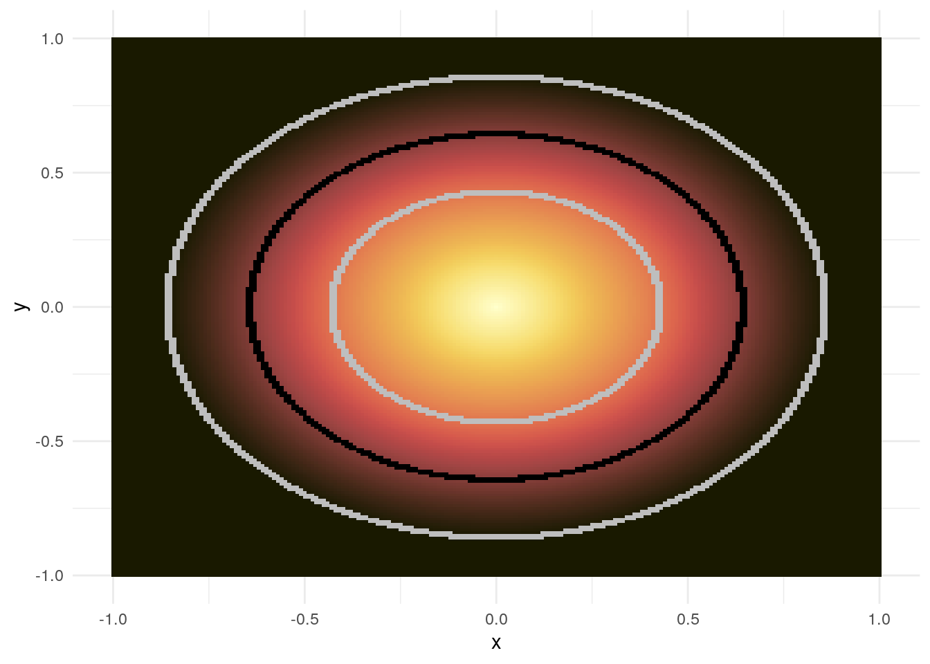
Figure 2.1: Example for a Z-plot: the $L_2$-norm

Any value above $4$ is now simply black which allows the plot to be compared across outlier detection algorithms as the colourbar remains constant. Furthermore, the inner gray circle refers to a threshold of $2$ whereas the outer gray circle refers to a threshold of $4$. The black circle in the middle corresponds to the value $3$. These are intended to visualize the outlier areas according to these three thresholds more clearly. Together, the Z-plot provides a good first look into the results of a certain outlier detection algorithm in two dimensions. We will therefore now discuss two-dimensional example data.

2.4 Evaluation of outlier detection algorithms

The discussion of anomaly benchmark datasets by Emmott et al. (2015) has a few implications for the evaluation of algorithms in this report: firstly, they point out that artificial data is almost always too simple and therefore not fit for a fair evaluation of outlier detection algorithms. They therefore advocate constructing benchmark data for this evaluation by modifying real datasets. In terms of characterizing these datasets, they identify four problem dimensions of anomaly detection:

point difficulty: how different are the outliers from the normal data points?
semantic variation: how different are the processes which create the different outliers? If many outliers are generated by the same process, this patterns might be captured by the algorithm which would yield unfavorable results.
relative frequency: how many data points are anomalies of interest?
feature relevance: how many of the feature dimensions are relevant/irrelevant for the task at hand?

The scope of this report is too narrow to include a detailed evaluation of the different algorithms. Instead, I will refer to other evaluations talk about influences of these four dimensions where they are evident. As a small visualization of the algorithms, I will introduce four datasets with different difficulties and outlier patterns. These can be seen in figure 2.2.

## Warning: `as_tibble.matrix()` requires a matrix with column names or a `.name_repair` argument. Using compatibility `.name_repair`.
## This warning is displayed once per session.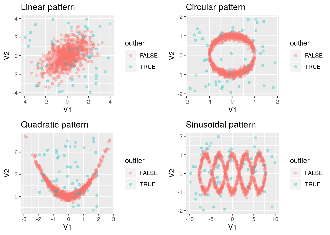

Figure 2.2: Example datasets

In the following chapters, I will distinguish outliers and normal data points by shape.

Clearly, these datasets represent different levels of difficulty – regarding the sinusoidal pattern, there might not even be accordance on the outliers between humans. Furthermore, I do not claim that these datasets represent a fair evaluation of the algorithms. They are only intended as simple examples of application. I will therefore not report the detection accuracy as this would implicitly rank the algorithms without a proper methodology. I also point out that the linear, circular and quadratic patterns are very difficult in terms of their little semantic variation.

References

Aggarwal, Charu C. 2017. Outlier Analysis. Springer Publishing Company, Incorporated.

Dempster, A P, N M Laird, and D B Rubin. 1977. “Maximum Likelihood from Incomplete Data via the EM Algorithm.” Journal of the Royal Statistical Society. Series B (Methodological) 39 (1). [Royal Statistical Society, Wiley]: 1–38. http://www.jstor.org/stable/2984875.

Deutsch, P. 1996. “DEFLATE Compressed Data Format Specification version 1.3.” https://doi.org/10.17487/rfc1951.

Emmott, Andrew, Shubhomoy Das, Thomas G Dietterich, Alan Fern, and Weng-Keen Wong. 2015. “Systematic Construction of Anomaly Detection Benchmarks from Real Data.” CoRR abs/1503.0. http://arxiv.org/abs/1503.01158.

Pedersen, Thomas Lin, and Fabio Crameri. 2018. scico: Colour Palettes Based on the Scientific Colour-Maps. https://cran.r-project.org/package=scico.