Chapter 4 Nonlinear extensions
4.1 Kernel PCA
4.1.1 Motivation
The greatest limitations of the methods presented in the last chapter had been their linearity. We may adress this issue by non-linear transformations of the variables. This is popular, for instance, with classical regression methods, as well. We therefore define a transformation
\[ \Phi: \mathbb{R}^p\to \mathbb{R}^q, X\mapsto \Phi(X). \]
Example 4.1 A common example would be a polynomial transformation, e.g.
\[ \Phi(X_1,\dotsc, X_p):=(X_1,X_1^2,X_1^3,\dotsc, X_p, X_p^2, X_p^3). \]We can now define the kernel PCA on \(X\) as a linear PCA on \(\Phi(X)\), as such a method would be able to capture non-linearities. However, computational limits come into mind: \(\Phi(X)\) is only required to compute \(\Phi(X)^T\Phi(X)\) which is only required to compute the principal components. For this reason, there is a more efficient way to compute the kernel PCA.2
The following proposition is the key to the solution:
Proposition 4.1 Consider the principal components
\[ XX^T=QM^2Q^T, Q,M\in\mathbb{R}^{n\times n}, Q^TQ=I, \]
and
\[ X^TX=P\Lambda^2P^T, P,\Lambda\in\mathbb{R}^{p\times p}, P^TP=I. \]
- For all \(1\le i\le p\), \(\Lambda_{ii}=M_{ii}\) and if \(i>p\), \(M_{ii}=0\),
- For all \(1\le k\le p\), the first \(k\) columns of \(QM\) correspond to the first \(k\) principal components. Columns \(p+1\) to \(n\) of \(QM\) are zero.
This proposition essentially yields that we can compute the PCA with \(XX^T\) alone. The kernel trick uses that fact by computing
\[ K(X):=\Phi(X)\Phi(X)^T \]
directly from \(X\) instead of computing \(\Phi(X)\) before the analysis. \(K\) is called the kernel.
4.1.2 Definition
In order to define kernel PCAs, we need to consider what properties \(K\) must possess. As principal component analysis only works on positively semi-definite matrices, we define a kernel as a function which only yields positively semi-definite matrices.
We can therefore define the kernel PCA in the following way:
Definition 4.1 Consider observations \(X\in\mathbb{R}^n\) and a kernel \(K:\mathbb{R}^n\to\mathbb{R}^{n\times n}\). Outlier detection using kernel PCA is defined by applying principal component analysis to
\[ K(X)=P\Lambda^2P^T. \]
which results in the nonlinear principal components \(T_1,\dotsc,T_m\) where \(m\le n\) is chosen such that \(\Lambda_{m+1}=0\). The outlier score is then defined by
\[ \sum_{k=1}^m\Lambda_{k}^{-2}T_k^2. \]The great advantage of such a definition is that we do not actually have to consider the nonlinear transformation of \(X\). Instead, we determine an appropriate similarity matrix which provides an easy extension of the kernel PCA to cases where \(X\) is not numeric. In practice, examples of popular kernels are
- polynomial kernels: \((X_i\cdot X_j+c)^h, c\in\mathbb{R},h\in \mathbb{N}\)
- \(c=.5\) and \(h=2\) would yield the square transformation \(X_k\mapsto (X_k, X_k^2)\)
- \(c=0\) and \(h=1\) would yield the ordinary dot product similarity matrix
- Gaussian kernels: \(\exp\left(-\frac{|X_i-X_j|^2}{\sigma^2}\right)\)
- Sigmoid kernels: \(\tanh\left(\kappa X_i\cdot X_j-\delta\right)\).
The package kernlab (Karatzoglou et al. 2004) implements kernel PCA in R.
- Compute the kernel PCA using
kernlab::kpca. The kernel is provided by an appropriate string to the argumentkerneland the parameters of the kernel are provided to the argumentkpar, e. g.:pca <- kernlab::kpca( ~ V1 + V2, data = data, kernel = "polynomial", kpar = list(c = 0.5, h = 2)). - Predict the principal components using
predict, e. g.pcs <- predict(pca, data) - Compute the outlier score, e. g.:
pcs ^ 2 %*% eig(pca) ^ (-2).
4.1.3 Example application
In the example application, we will consider the following two kernels:
- Square kernel: \(K(X_i,X_j):=(X_i\cdot X_j+0.5)^2\)
- Gaussian kernel: \(\exp(-\frac{|X_i-X_j|^2}{\sigma^2})\)
By default, \(\sigma\) is set as \(0.1\), so we will use that parameter value.
We will first consider results regarding the linear pattern, as shown in figure 4.1.
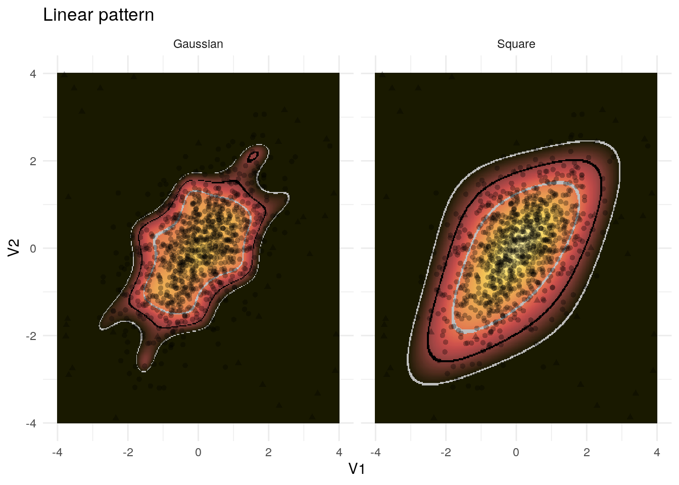
Figure 4.1: Example application of the kernel PCA to the linear pattern
The Gaussian kernel is too restrictive with respect to the linear pattern and both the Gaussian and the polynomial kernel again regard both directions as important where the pattern is actually given by the line.
Both methods fare quite well with the circular pattern in 4.2.
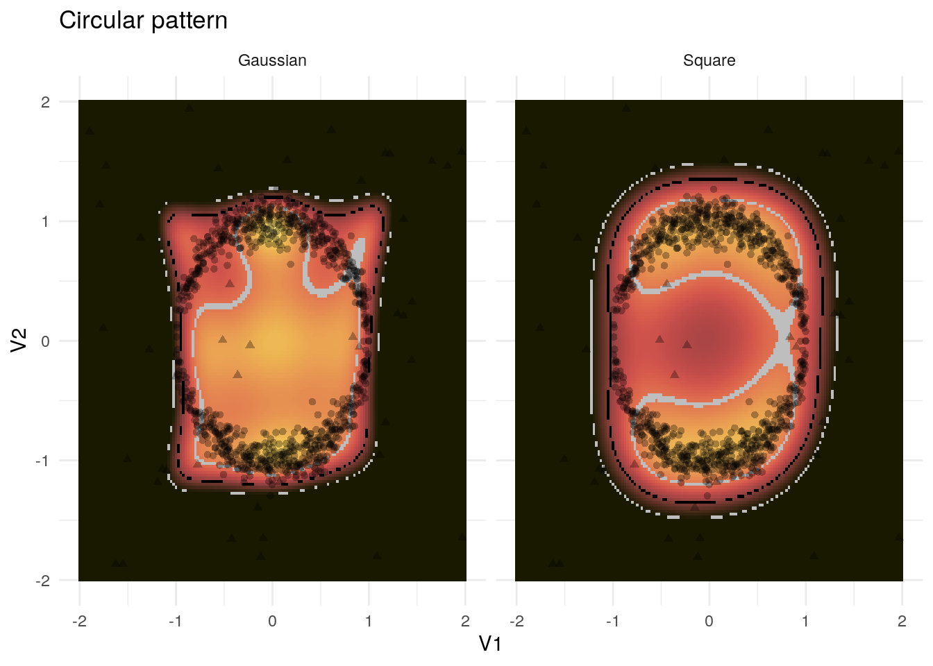
Figure 4.2: Example application of the kernel PCA to the circular pattern
Even though some inliers might be classified as outliers according to the threshold of 2 standard deviations, any other threshold recognizes the inliers. The Gaussian kernel even recognizes that the points within the circle should be classified as outliers, as well. On the whole, both methods results correspond to our intuition and are fairly strict.
In contrast, the Gaussian kernel is too strict with respect to the quadratic pattern in 4.3.
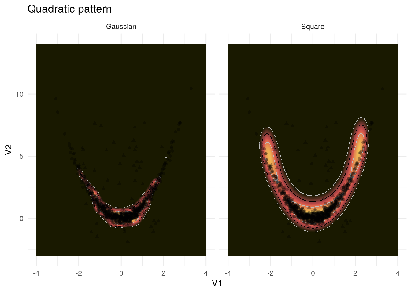
Figure 4.3: Example application of the kernel PCA to the quadratic pattern
However, the polynomial kernel captures the pattern almost perfectly.
Finally, both methods struggle with the sinusoidal pattern in 4.4. The polynomial seems insufficiently complex for this pattern whereas the more local Gaussian kernel does not recognize the overall pattern but only some denser points. The latter is, on the whole, too restrictive, however.
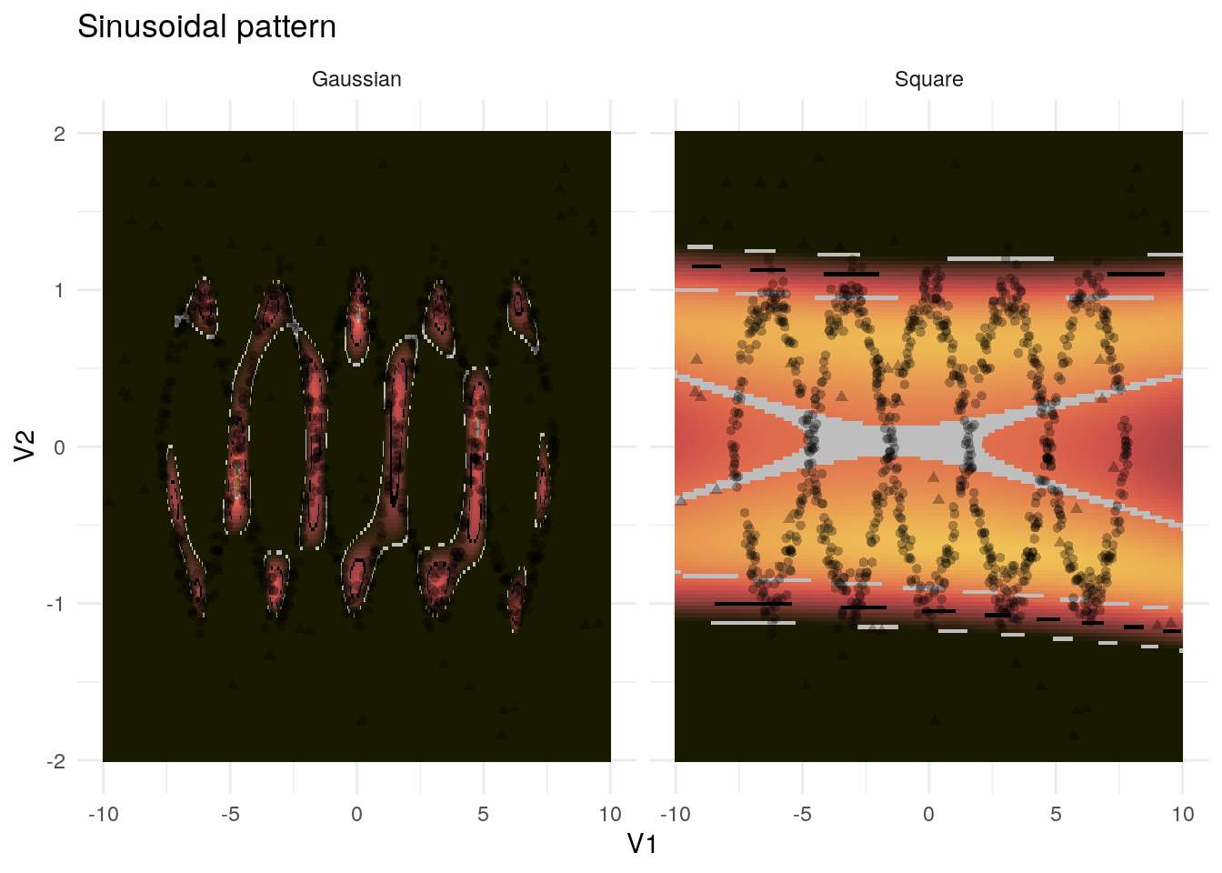
Figure 4.4: Example application of the kernel PCA to the sinusoidal pattern
These examples demonstrate that kernel PCAs can yield powerful results but still need to be assessed carefully. Fitting the hyperparameters and using certain evaluation criteria can help ensure a good result. In particular the quadratic kernel seems to be adept at handling nonlinear patterns which are not too complex.
4.1.4 Discussion
In summary, the great flexibility is the decisive advantage of kernel PCA. This method, together with the right kernel, can recognize and handle arbitrary data. Such flexibility, however, has a downside, as well. Due to the many hyperparameters, the method is susceptible to overfitting. Moreover, it is more difficult to fit such a model compared to a linear model which is relatively easy to understand and apply.
Another advantage which comes with the kernel trick is that any similarity measure can be used for kernel PCA as long as it yields a positive semi-definite matrix. This means that kernel PCA can be applied to topics as diverse as graph analysis, spatiotemporal analysis and text analysis.
4.2 Neural networks
I will conclude with a short excursion to outlier detection using neural networks.
Neural networks are a Machine Learning algorithm which is adept at approximating complex, non-linear patterns. Their application to outlier detection can well be motivated by considerations in the field of data compression. We compress data by identifying its decisive properties and attempting to summarize it by as few numbers as possible. For instance our perception summarizes any colour by three numbers: its redness, blueness and greenness. Three numbers are therefore sufficient to describe our perception of any colour. These summaries are often nonlinear which is why neural networks are suitable for handling them. Broadly speaking, neural networks consist of several layers of nodes where a weighted sum of all the nodes in one layer feeds into the node of the next layer. Any layer therefore only depends on the values in the layer before.3
The idea of outlier detection using neural networks is therefore the following: we map the input layer (i. e. all variables) through several intermediate layers to the mid-layer which contains of a lower number of nodes. Then we reflect this architecture and finally attempt to predict the same variables from the initial variables by following the backpropagation algorithm. The better we perform at predicting the input from the input the better our compression using the mid-layer works. On the other hand, those observations which cannot be predicted very well apparently do not adhere to the general pattern.
In R, neural networks can, for instance, be fitted using the package keras. (Allaire and Chollet 2018) Due to the many hyperparameters such as number of layers and number of nodes in each layer, fitting a neural network is a complex undertaking which goes beyond the scope of this report. An introduction to fitting neural networks can be found in section 10.7 of Aggarwal (2015).
I will conclude this report by revisiting the introduction in which we discussed outlier detection using predictive coding in the brain. Interestingly, a recent paper by Whittington and Bogacz (2017) demonstrated equivalency of neural networks and predictive coding under certain conditions. This has two implications: on the one hand, neural networks might bring us closer to understanding how our brain detects outliers. This is more important in outlier detection than in other statistical fields as outlier detection is more vaguely defined and depends more strongly on human intuition. On the other hand, predictive coding might contain new suggestions for complex probablistic outlier detection methods.
References
Aggarwal, Charu C. 2015. Data Mining. 1st ed. Springer International Publishing.
Allaire, J J, and François Chollet. 2018. keras: R Interface to ’Keras’. https://cran.r-project.org/package=keras.
Karatzoglou, Alexandros, Alex Smola, Kurt Hornik, and Achim Zeileis. 2004. “kernlab – An S4 Package for Kernel Methods in R.” Journal of Statistical Software 11 (9): 1–20. http://www.jstatsoft.org/v11/i09/.
Whittington, James C. R., and Rafal Bogacz. 2017. “An Approximation of the Error Backpropagation Algorithm in a Predictive Coding Network with Local Hebbian Synaptic Plasticity.” Neural Computation 29: 1229–62. https://doi.org/10.1162/NECO.